
Most explanations of star and snowflake schemas use the same toy: a Sales table, a Product table, a Store table and a diagram with five boxes. It shows the shapes, but not what happens when real data arrives: guest checkouts with no customer, discounts stored in a separate table, test orders, a customer who changes their email consent halfway through the year.
This guide builds both shapes from a real Shopify store, using the table and column names Shopify data has when Weld syncs it to your warehouse. Every query in it has been run against sample Shopify orders.
The short answer. A star schema puts one fact table in the middle and joins it to wide, flat dimension tables. A snowflake schema splits those dimensions into chains of smaller, normalised tables. Both hold the same information. In a modern columnar warehouse such as BigQuery or Snowflake, use a star by default, snowflake a dimension only when a hierarchy is shared and maintained on its own, and add one big wide table on top when a tool wants a single table.
Facts and dimensions, using one Shopify order
Start with a single order. Order #1042 was placed on 14 March 2026 by a customer in Copenhagen who is subscribed to email. It has two lines: two Merino Crew sweaters in L / Navy with a 24.00 discount, and one Canvas Tote with a 3.50 discount.

A fact table records events you measure. Each row is one event at a fixed level of detail, and its columns are either keys or numbers you add up: quantity, gross sales, discount, net sales.
A dimension table describes the things those events involve. Each row is one customer, one product variant or one day, and its columns are the attributes you filter and group by: country, product type, weekday.
| Fact table | Dimension table | |
|---|---|---|
| One row is | One event: an order line, a payment, a session | One thing: a customer, a product, a date |
| Columns | Foreign keys plus numeric measures | A key plus descriptive attributes |
| Shape | Narrow and long, grows with every order | Wide and short, grows with your catalogue and customer base |
| Changes | Appended to, rarely updated | Attributes change over time (see SCD Type 2 below) |
| In SQL you | sum(), count(), avg() it | group by and where on it |
| Shopify example | fct_order_line | dim_customer, dim_product, dim_date |
Three details in this one order matter for every model built on it.
The grain is the order line, not the order. The Kimball Group calls declaring the grain "the pivotal step in a dimensional design", because it fixes what one row means. Shopify stores the order header in order and the products in order_line. If the fact table were one row per order, product would not fit in it: order #1042 contains two products. At line grain, both products get a row and order-level questions are still a count(distinct order_id) away.
The order number is a degenerate dimension. #1042 is a useful key to filter and group by, but there is nothing else to say about it once the customer, date and products have their own tables. Kimball's term for a key like that is a degenerate dimension: it lives on the fact table with no dimension table behind it.
Not every key has a match. Guest checkouts have no customer_id. Join the fact to dim_customer with a left join, or add an "unknown customer" row to the dimension, or those orders disappear from every report grouped by customer.
Star schema: the model and the SQL
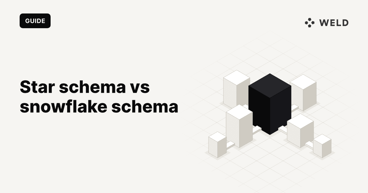
A star schema joins the fact table directly to each dimension. Every descriptive attribute about a product, including its type and vendor, sits in one flat dim_product row. Here are both shapes from the same Shopify tables, side by side:

The SQL below is BigQuery. It reads the raw tables Weld syncs from Shopify (order, order_line, discount_allocation, customer, customer_address, product, product_variant) and writes four tables to a gold dataset.
The dimensions
dim_customer flattens the customer and their default address into one row:
1create or replace table
2    gold.dim_customer as
3select
4    c.id as customer_id
5  , c.email
6  , c.first_name
7  , c.last_name
8  , c.email_marketing_consent_state
9  , a.country_code
10  , a.country
11  , a.city
12  , date(c.created_at) as customer_since
13from
14    shopify.customer as c
15    left join shopify.customer_address as a on a.customer_id = c.id
16    and a.is_default;
dim_product is one row per variant, because orders reference variants, with the product's title, type and vendor copied onto every variant:
1create or replace table
2    gold.dim_product as
3select
4    v.id as product_variant_id
5  , v.sku
6  , p.title as product_title
7  , v.title as variant_title
8  , p.product_type
9  , p.vendor
10  , p.status as product_status
11  , v.price as list_price
12from
13    shopify.product_variant as v
14    join shopify.product as p on p.id = v.product_id;
dim_date does not come from Shopify at all. Generate it once, so every report can group by month or weekday without date functions in every query:
1create or replace table
2    gold.dim_date as
3select
4    d as date_day
5  , extract(
6        year
7        from
8            d
9    ) as year
10  , extract(
11        quarter
12        from
13            d
14    ) as quarter
15  , format_date('%Y-%m', d) as year_month
16  , format_date('%A', d) as day_name
17  , extract(
18        dayofweek
19        from
20            d
21    ) in (1, 7) as is_weekend
22from
23    unnest (generate_date_array('2020-01-01', '2030-12-31')) as d;
The fact table
One row per order line. Line discounts live in Shopify's discount_allocation table, so they are summed per line first. Test orders and cancelled orders are dropped here, once, instead of in every report:
1create or replace table
2    gold.fct_order_line as
3with
4    line_discounts as (
5        select
6            order_line_id
7          , sum(amount_set_shop_money_amount) as discount
8        from
9            shopify.discount_allocation
10        group by
11            order_line_id
12    )
13select
14    ol.id as order_line_id
15  , o.id as order_id
16  , o.name as order_name -- degenerate dimension, e.g. #1042
17  , o.customer_id
18  , ol.variant_id as product_variant_id
19  , date(o.processed_at) as order_date
20  , ol.quantity
21  , ol.price * ol.quantity as gross_sales
22  , coalesce(ld.discount, 0) as discount
23  , ol.price * ol.quantity - coalesce(ld.discount, 0) as net_sales
24from
25    shopify.order_line as ol
26    join shopify.`order` as o on o.id = ol.order_id
27    left join line_discounts as ld on ld.order_line_id = ol.id
28where
29    not o.test
30    and o.cancelled_at is null;
This is a modelling example, not a finance report. Refunds, returns, order edits and shipping are left out to keep the shape visible. If you need numbers that match Shopify's own sales report, build the fact from the order agreement tables as described in Shopify dbt models: a production sales report that matches the admin. The star around it stays the same.
date(o.processed_at) also gives you the UTC date. If your store reports in another timezone, convert first, for example date(o.processed_at, 'Europe/Copenhagen').
The query
Net sales by month, product type and customer country. Three joins, each one hop from the fact:
1select
2    d.year_month
3  , p.product_type
4  , c.country
5  , sum(f.quantity) as units
6  , sum(f.net_sales) as net_sales
7from
8    gold.fct_order_line as f
9    join gold.dim_date as d on d.date_day = f.order_date
10    join gold.dim_product as p on p.product_variant_id = f.product_variant_id
11    left join gold.dim_customer as c on c.customer_id = f.customer_id
12where
13    d.year = 2026
14group by
15    1
16  , 2
17  , 3
18order by
19    1
20  , 2
21  , 3;
Anyone who can read the diagram can write this query, and a BI tool or an AI agent can generate it from the table names alone. That is most of the case for a star.
Snowflake schema: the same data, normalised
A snowflake schema takes each dimension and splits out its hierarchies into their own tables. Product variant points to product, product points to product type. Customer points to country. Date points to month. Nothing is lost, and nothing is added: Kimball's own definition notes that a flattened dimension "contains exactly the same information as a snowflaked dimension."
The product chain looks like this:
1create or replace table
2    gold_sf.dim_product_variant as
3select
4    id as product_variant_id
5  , product_id
6  , sku
7  , title as variant_title
8  , price as list_price
9from
10    shopify.product_variant;
11
12create or replace table
13    gold_sf.dim_product as
14select
15    id as product_id
16  , title as product_title
17  , product_type
18  , vendor
19  , status as product_status
20from
21    shopify.product;
22
23create or replace table
24    gold_sf.dim_product_type as
25select distinct
26    product_type
27from
28    shopify.product;
dim_country (from customer_address), a slimmer dim_customer that keeps only country_code, and a dim_month that dim_date points to follow the same pattern. The fact table does not change.
The same question now takes seven joins, because month, product type and country are each two or three hops from the fact. The product type, customer and country joins are left joins, so a product with no type or a guest order still counts:
1select
2    m.year_month
3  , pt.product_type
4  , co.country
5  , sum(f.quantity) as units
6  , sum(f.net_sales) as net_sales
7from
8    gold.fct_order_line as f
9    join gold_sf.dim_date as d on d.date_day = f.order_date
10    join gold_sf.dim_month as m on m.year_month = d.year_month
11    join gold_sf.dim_product_variant as v on v.product_variant_id = f.product_variant_id
12    join gold_sf.dim_product as p on p.product_id = v.product_id
13    left join gold_sf.dim_product_type as pt on pt.product_type = p.product_type
14    left join gold_sf.dim_customer as c on c.customer_id = f.customer_id
15    left join gold_sf.dim_country as co on co.country_code = c.country_code
16where
17    m.year = 2026
18group by
19    1
20  , 2
21  , 3
22order by
23    1
24  , 2
25  , 3;
We ran both queries against the same sample orders and they return the same rows. The snowflake is not more correct. It is more tables to write, document and join.
When a snowflaked dimension earns its place
A snowflake is the right call for a specific dimension, rarely for a whole model:
- The hierarchy has attributes of its own that someone maintains. If merchandising owns a mapping from Shopify's free-text
product_typeto departments, margin targets and buyers, that mapping is a table. Joiningdim_productto it is a snowflake, and that is fine. - The same hierarchy is shared by several dimensions. Country attributes such as region, VAT zone or currency can be used by customers, locations and suppliers alike. One
dim_countrykeeps them consistent. - A dimension is very large and one attribute group changes much faster than the rest. Splitting it lets you rebuild the fast-changing part without rewriting the whole dimension.
Even then, you can join the outrigger into a flat view for the people and tools that query it, and keep the normalised tables underneath.
Star vs snowflake schema compared
| Star schema | Snowflake schema | |
|---|---|---|
| Dimensions | One flat, wide table per dimension | Split into chains of normalised tables |
| Joins for month × product type × country | 3 | 7 |
| Storage in a columnar warehouse | Repeated text in dimensions compresses well; dimensions are small next to facts | Slightly less, rarely a difference you will see on the bill |
| Query speed | Fewer joins; the shape warehouses and BI engines are tuned for | More joins; often close in practice on modern engines |
| Writing queries | Easy for people, BI tools and AI agents | Needs the join path for every attribute |
| Maintenance with ELT | Each dimension is rebuilt by one query | More models, but each one is small |
| Best for | Reporting, BI, semantic layers, agents | Shared hierarchies maintained on their own |
Most comparisons still list "uses less storage" as the snowflake schema's main advantage. That made sense for row-based databases with expensive disks. In a columnar warehouse, a product_type value repeated on every variant row compresses to very little, and the dimension tables are tiny next to the fact table. The fact table, which is identical in both shapes, is where the storage and scan costs are.
Which to pick in BigQuery or Snowflake today, and one big table
Columnar warehouses changed the trade-off in two ways. Wide tables are cheap, because a query only reads the columns it uses. And joins to small dimensions are fast, so the star does not cost much at query time either.
So why not skip dimensions entirely and build one big table (OBT), with every attribute copied onto every order line?
1create or replace table
2    gold.obt_order_line as
3select
4    f.*
5  , d.year_month
6  , d.day_name
7  , p.sku
8  , p.product_title
9  , p.product_type
10  , p.vendor
11  , c.email_marketing_consent_state
12  , c.country_code
13from
14    gold.fct_order_line as f
15    join gold.dim_date as d on d.date_day = f.order_date
16    join gold.dim_product as p on p.product_variant_id = f.product_variant_id
17    left join gold.dim_customer as c on c.customer_id = f.customer_id;
Now the earlier report is a group by on one table. Google's own guidance is more measured than "always denormalise". The BigQuery documentation on nested and repeated fields (updated 27 October 2026) says that "star schemas are typically optimized schemas for analytics", and that denormalising further may not make queries significantly faster. Where it does suggest denormalising, it recommends nested and repeated fields, for example the order lines as an array inside one order row, over flattening everything.
Snowflake can also skip joins a query does not need. If you declare primary and foreign keys with the RELY property, Snowflake can eliminate a join to a dimension whose columns the query does not select. Databricks SQL does the same with RELY constraints. Both depend on you guaranteeing the keys are actually unique, since neither enforces them on standard tables.
One big table is fine when:
- one team, one dashboard tool, one subject: an ecommerce sales dashboard on order lines
- the tool wants a single table, such as a spreadsheet export, a reverse ETL sync or a simple BI connector
- dimension attributes rarely change, or you only ever want their current value
A star is still worth it when:
- More than one fact shares a dimension. Orders, refunds, ad spend and sessions all need the same
dim_productanddim_date. Kimball calls these conformed dimensions: define product once, and a report can line up sales and ad spend by product type on the same rows. Four wide tables each carrying their own copy of product attributes drift apart. - Attributes change. Renaming a product type in a star rebuilds a few thousand dimension rows. In a wide table it rewrites every order line that ever had that type.
- You need history. An SCD Type 2 dimension needs a point-in-time join, which only exists if the dimension is a table of its own (next section).
- Something other than a person writes the SQL. Semantic layers, BI models and AI agents work best with a small number of well-named tables and obvious joins. A star is the shape they expect.
In practice the answer is usually both: model a star in gold, and publish a wide table or view on top of it for the tools that want one. The star is the source of truth, the wide table is a convenience that can be rebuilt from it at any time.
SCD Type 2 dimensions and the medallion gold layer
dim_customer above holds each customer's current state. If a customer subscribed to email in March, every order they placed in February now also looks like it came from a subscriber. That is a slowly changing dimension problem, and Type 2 solves it: keep one row per version of the customer, each with the period it was valid.
Weld can keep that history for you. Turn on a history table for Shopify's customer table, and every changed version of a customer lands in customer__history, with the same columns as customer, including _weld_synced, the time Weld synced that version. Turning the history into a Type 2 dimension is one query:
1create or replace table
2    gold.dim_customer_scd2 as
3with
4    versions as (
5        select
6            id as customer_id
7          , email
8          , email_marketing_consent_state
9          , updated_at
10        from
11            shopify.customer__history
12        where
13            updated_at is not null
14        qualify
15            row_number() over (
16                partition by
17                    id
18                  , updated_at
19                order by
20                    _weld_synced desc
21            ) = 1
22    )
23select
24    to_hex(
25        md5(
26            concat(
27                cast(customer_id as string)
28              , cast(updated_at as string)
29            )
30        )
31    ) as customer_key
32  , customer_id
33  , email
34  , email_marketing_consent_state
35  , updated_at as valid_from
36  , lead(updated_at) over (
37        partition by
38            customer_id
39        order by
40            updated_at
41    ) as valid_to
42  , lead(updated_at) over (
43        partition by
44            customer_id
45        order by
46            updated_at
47    ) is null as is_current
48from
49    versions;
customer_key is a surrogate key: one value per version, where customer_id is the same for all versions of a customer. The fact table still carries customer_id, and the join picks the version that was valid when the order was processed:
1select
2    c.email_marketing_consent_state as consent_when_ordered
3  , count(distinct f.order_id) as orders
4  , sum(f.net_sales) as net_sales
5from
6    gold.fct_order_line as f
7    join shopify.`order` as o on o.id = f.order_id
8    left join gold.dim_customer_scd2 as c on c.customer_id = f.customer_id
9    and o.processed_at >= c.valid_from
10    and (
11        o.processed_at < c.valid_to
12        or c.valid_to is null
13    )
14group by
15    1;
In our sample, the same customer's February order lands under NOT_SUBSCRIBED and the March order under SUBSCRIBED, which is the answer "how much revenue came from customers who were subscribed when they bought?" needs. Join to is_current instead when you want today's view of every customer. Both questions work against the same star, and neither works against a wide table that copied the consent state once.
For the incremental version, with a MERGE that closes and inserts versions, dbt snapshots, deletes and late rows, see SCD Type 2 in SQL.
Where the gold layer fits
In a medallion architecture, the star is the gold layer. Bronze holds Shopify's tables exactly as synced, including the history tables. Silver cleans them one table at a time: renames, types, test orders out, history deduplicated. Gold is where facts and dimensions are built, and where dashboards, a semantic layer or an AI agent read from. The SQL in this guide reads the raw tables straight into gold to stay short; in a real project the renames and the test-order filter move into silver.

Weld covers that whole path: it syncs Shopify into BigQuery, Snowflake or another warehouse, keeps the history tables, and runs the SQL or dbt models for silver and gold on a schedule after each sync. Our 5-stage framework splits gold further into core models and analytics models, which is a good home for the star (core) and the wide tables built on it (analytics).
Dimensional modeling and the Kimball method in four steps
Everything above follows Kimball's four-step design process, which still works when the warehouse is BigQuery and the source is Shopify:
- Select the business process. Selling products online.
- Declare the grain. One row per order line.
- Identify the dimensions. Customer, product variant, date, plus the order number as a degenerate dimension.
- Identify the facts. Quantity, gross sales, discount, net sales.
Do the next business process the same way, say refunds or ad spend, and reuse the same dimensions. That reuse, more than any choice between star and snowflake, is what keeps numbers consistent across reports. For more on the vocabulary, see our data modelling entry.
FAQ
A star schema joins one fact table directly to flat, denormalised dimension tables. A snowflake schema normalises those dimensions into chains of smaller tables, such as product to product type, or customer to country. They hold the same information; the snowflake needs more joins to read it.
A star schema is usually faster and never slower to write, because each attribute is one join from the fact table. In columnar warehouses like BigQuery and Snowflake, the difference is often small, since dimension tables are small and joins to them are cheap. Fewer joins also make queries easier for BI tools and AI agents to generate correctly.
Very little in a modern warehouse. Columnar storage compresses repeated values in a dimension column, and dimensions are small compared with the fact table, which is identical in both designs. Storage was a stronger argument for row-based databases.
A fact table records events at a fixed grain, such as one row per Shopify order line, with keys and numeric measures like quantity and net sales. A dimension table describes the things in those events, such as one row per customer, product variant or day, with attributes you filter and group by.
Use one big table for a single subject and tool, such as an ecommerce sales dashboard, when attributes rarely change. Keep a star underneath when several fact tables share dimensions, when you need history from SCD Type 2 dimensions, or when a semantic layer or AI agent queries the model. Many teams publish a wide table built from the star.
Yes, and most real models do. Keep dimensions flat by default and snowflake only the hierarchies that are shared or maintained on their own. A model with several fact tables sharing the same dimensions is sometimes called a galaxy schema or fact constellation.
It is Ralph Kimball's approach to dimensional modeling: select a business process, declare the grain, identify the dimensions, identify the facts, and reuse conformed dimensions across fact tables. The star schema is its standard output.
Additional resources
- Slowly changing dimensions (SCD): types 1 to 4 and history tables
- SCD Type 2 in SQL: MERGE, dbt snapshots and history tables
- Medallion architecture: bronze, silver and gold layers explained
- A 5-stage framework for data modeling
- Shopify dbt models: a production sales report
- Shopify sales report in SQL
- History tables in Weld
- Kimball Group: dimensional modeling techniques
- BigQuery: use nested and repeated fields
- Snowflake: join elimination